This document introduces you to rminka basic set of tools, and shows you how to apply them to obtain your desired information. Once you’ve installed, read vignette(“rminka”) to learn more.
- Project Queries
Project-related functions will be illustrated using the project Biomarató Tarragona 2025.
● mnk_proj_byname()
Initially, only the project name is known, so a search is performed
to retrieve the corresponding project ID. This is done with
mnk_proj_byname(). Here we use the query “biomarato
2025”.
prj_names <- mnk_proj_byname("biomarato 2025")

prj_names
#> # A tibble: 5 × 8
#>      id title      place_id slug  created_at updated_at project_type description
#>   <int> <chr>         <int> <chr> <chr>      <chr>      <chr>        <chr>
#> 1   417 BioMARató…      244 biom… 2025-03-2… 2026-05-0… collection   "La BioMAR…
#> 2   418 BioMARató…      245 biom… 2025-03-2… 2026-05-0… collection   "La BioMAR…
#> 3   419 BioMARató…      249 biom… 2025-03-2… 2026-05-0… collection   "La BioMAR…
#> 4   420 BioMARató…      248 biom… 2025-03-2… 2026-05-0… collection   "La BioMAR…
#> 5   424 BioMARato…      701 biom… 2025-04-0… 2025-12-1… collection   "Descobre …

# For this example

prj_names[,c(1:2)]
#> # A tibble: 5 × 2
#>      id title
#>   <int> <chr>
#> 1   417 BioMARató 2025 (Catalunya)
#> 2   418 BioMARató 2025 (Girona)
#> 3   419 BioMARató 2025 (Tarragona)
#> 4   420 BioMARató 2025 (Barcelona)
#> 5   424 BioMARatona 2025
● mnk_proj_info()
Once the project ID is known, detailed information can be retrieved
with mnk_proj_info(). For the Biomarató Tarragona 2025, the
project ID is 419.
prj_info <- mnk_proj_info(419)

prj_info
#> # A tibble: 1 × 7
#>      id title               created_at subscrib_users place_id slug  description
#>   <int> <chr>               <chr>               <int>    <int> <chr> <chr>
#> 1   419 BioMARató 2025 (Ta… 2025-03-2…             23      249 biom… La BioMARa…
● mnk_proj_user()
Users explicitly subscribed to a project can be retrieved with
mnk_proj_user() using the project ID
prj_user <- mnk_proj_user(419)

prj_user
#> # A tibble: 23 × 16
#>       id login          name              created_at          observations_count
#>    <int> <chr>          <chr>             <dttm>                           <int>
#>  1     4 xasalva        "xavi salvador c… 2021-04-16 10:44:11              83172
#>  2     6 ramonservitje  ""                2022-04-16 15:47:14               1259
#>  3    11 jaume-piera    "Jaume Piera"     2022-04-18 15:45:37              11332
#>  4    12 sonialinan      NA               2022-04-19 12:53:18                410
#>  5    13 adrisoacha     "Karen Soacha"    2022-04-21 09:40:57                592
#>  6    52 joselu_00      "José Luís Guijo… 2022-05-10 13:38:20                404
#>  7   159 jaumesaltiveri "Jaume Saltiveri" 2022-07-17 13:30:45                  2
#>  8   166 anomalia       "anomalia"        2022-07-19 07:56:08                 23
#>  9   197 peixderoca24   "Guillem Mayor S… 2022-08-08 12:58:18               4546
#> 10   219 ealcaniz       "Edu Alcaniz"     2022-08-27 15:52:52              27917
#> # ℹ 13 more rows
#> # ℹ 11 more variables: identifications_count <int>, species_count <int>,
#> #   activity_count <int>, journal_posts_count <int>, orcid <chr>,
#> #   icon_url <chr>, site_id <int>, roles <list>, spam <lgl>, suspended <lgl>,
#> #   universal_search_rank <int>
Note: The simplest way to retrieve all participants in a project —
including those who are not subscribed — is to download the project’s
observations with mnk_proj_obs() and then extract the
unique values of user_login. Each observation includes the observer’s
login, so the set of distinct logins corresponds to the project’s
participants.
If the project lasts only one year, or if you are only interested in
the participants from a single month, a single function call is
sufficient. For example, project 419 ran in 2025, so all its
observations can be obtained with
mnk_proj_obs(419, year = 2025):
# 1. Download all observations for the project in may 2025

obs_2025 <- mnk_proj_obs(419,year=2025, mont=5, quiet = TRUE)

# 2. Extract the unique participants

participants_may_2025 <- obs_2025 %>%
  distinct(user_login) %>%
  arrange(user_login)

participants_may_2025
#> # A tibble: 30 × 1
#>    user_login
#>    <chr>
#>  1 aci
#>  2 albertvim
#>  3 allbluediving
#>  4 bertinhaco
#>  5 biosub
#>  6 elibonfill
#>  7 elisenda_casabona
#>  8 evararo
#>  9 francesca
#> 10 hectorserranocereijo
#> # ℹ 20 more rows
● mnk_proj_obs()
Returns all observations for a project within a selected year, and
optionally within a specific month. For the Biomarató Tarragona 2025
(project ID 419), observations for the entire year are obtained with
mnk_proj_obs(419, year = 2025), while observations for a
single month — for example, May — are obtained with
mnk_proj_obs(419, year = 2025, month = 5).
prj_obs <- mnk_proj_obs(419, year= 2025, month=5)
#> --- STARTING DOWNLOAD FOR MONTH: May 2025 ---
#>
#> --- Evaluating month: May 2025 ---
#> The month of May has 1173 records.
#>  -> Total <= 10,000. Downloading month in one go...
#>
#> --- FINISHING... ---
#> Download complete! A total of 1,173 records were obtained.

prj_obs[2:14]
#> # A tibble: 1,173 × 13
#>    observed_on  year month  week   day  hour created_at      updated_at latitude
#>    <chr>       <int> <int> <int> <int> <int> <chr>           <chr>         <dbl>
#>  1 2025-05-23   2025     5    21    23    11 2026-03-14T12:… 2026-03-1…     41.1
#>  2 2025-05-24   2025     5    21    24    19 2025-10-22T21:… 2025-10-2…     41.2
#>  3 2025-05-24   2025     5    21    24    19 2025-10-22T21:… 2025-10-2…     41.2
#>  4 2025-05-24   2025     5    21    24    19 2025-10-22T21:… 2025-10-2…     41.2
#>  5 2025-05-24   2025     5    21    24    19 2025-10-22T21:… 2025-10-2…     41.2
#>  6 2025-05-24   2025     5    21    24    19 2025-10-22T21:… 2025-10-2…     41.2
#>  7 2025-05-24   2025     5    21    24    19 2025-10-22T21:… 2025-10-2…     41.2
#>  8 2025-05-24   2025     5    21    24    19 2025-10-22T21:… 2025-11-0…     41.2
#>  9 2025-05-24   2025     5    21    24    18 2025-10-22T21:… 2025-10-2…     41.2
#> 10 2025-05-24   2025     5    21    24    18 2025-10-22T21:… 2025-10-2…     41.2
#> # ℹ 1,163 more rows
#> # ℹ 4 more variables: longitude <dbl>, positional_accuracy <int>,
#> # geoprivacy <chr>, obscured <lgl>● mnk_user_byname()
Initially, only an approximate name is known, so a search is performed to retrieve the corresponding user_login. For this example, we start with the query “xavi”, which returns a list of possible logins. The desired user — Xavier Salvador — is then selected from that list.
user_name <- mnk_user_byname("xavi")

user_name
#> # A tibble: 6 × 5
#>      id login             name            observations_count created_at
#>   <int> <chr>             <chr>                        <int> <dttm>
#> 1    47 xavi               NA                              6 2022-05-06 10:47:06
#> 2     4 xasalva           "xavi salvador…              83172 2021-04-16 10:44:11
#> 3  1178 xparellada        "Xavier Parell…                670 2023-10-31 09:07:52
#> 4   857 xavibou           "Xavi Bou"                    1087 2023-07-28 13:27:50
#> 5  1042 xavi-de-yzaguirre ""                             459 2023-09-26 13:18:42
#> 6 17242 xavisanjuan        NA                            390 2025-07-20 16:21:42
● mnk_user_info()
Once the user ID is known, detailed information can be retrieved with mnk_user_info(). For Xavier Salvador (login “xasalva”), the user ID is 4
user_info <- mnk_user_info(4)

user_info
#> # A tibble: 1 × 16
#>      id login name  created_at          observations_count identifications_count
#>   <int> <chr> <chr> <dttm>                           <int>                 <int>
#> 1     4 xasa… xavi… 2021-04-16 10:44:11              83172                420171
#> # ℹ 10 more variables: species_count <int>, activity_count <int>,
#> #   journal_posts_count <int>, orcid <chr>, icon_url <chr>, site_id <int>,
#> #   roles <list>, spam <lgl>, suspended <lgl>, universal_search_rank <int>
● mnk_user_proj()
mnk_user_proj() returns the projects to which a user is
explicitly subscribed, given the user ID. For Xavier Salvador (user ID
4), the list is obtained with mnk_user_proj(4).
Note: Projects in which a user has contributed observations but is not formally subscribed cannot be retrieved directly in R.
user_project <- mnk_user_proj(4)

user_project
#> # A tibble: 10 × 7
#>       id title                       description slug  icon  place_id created_at
#>    <int> <chr>                       <chr>       <chr> <chr>    <int> <chr>
#>  1   522 (Principal) Biodiverciutat… "Aquest pr… prin… http…       NA 2025-10-2…
#>  2   144 ANERIS - Biodiversitat D.C… "El projec… aner… http…      337 2023-06-0…
#>  3   312 ANERIS - Biodiversitat Llo… "El projec… aner… http…      416 2024-06-1…
#>  4   146 ANERIS - Biodiversitat UNI… "El projec… aner… http…      338 2023-06-0…
#>  5   177 ANERIS - Biodiversitat al … "El projec… aner… http…      361 2023-08-2…
#>  6   183 ANERIS - SASBA (Seguiment … "Descobrim… aner… http…      251 2023-10-0…
#>  7    44 Anthozoos del Barcelonés    "Estudi de… anth… http…       NA 2022-09-2…
#>  8   444 Arees verdes marines - Emp… "Aquest pr… aree… http…      712 2025-05-2…
#>  9   448 BIODIVERSIDAD MARINA BADIA… "Estudio d… biod… http…      714 2025-05-2…
#> 10   181 BM-PortSalvi                "El projec… bm-p… http…      367 2023-09-1…
● mnk_user_obs()
Returns all observations for a user within a selected year, and
optionally within a specific month. For Xavier Salvador (user ID 4),
observations for the entire year are obtained with
mnk_user_obs(4, year = 2025), while observations for a
single month, for example May, are obtained with
mnk_user_obs(4, year = 2025, month = 5).
user_obs <- mnk_user_obs(user_id= 4, year = 2025, month = 8)
#> --- STARTING DOWNLOAD FOR MONTH: August 2025 ---
#>
#> --- Evaluating month: August 2025 ---
#> The month of August has 2347 records.
#>  -> Total <= 10,000. Downloading month in one go...
#>
#> --- FINISHING... ---
#> Download complete! A total of 2,347 records were obtained.

user_obs
#> # A tibble: 2,347 × 27
#>        id observed_on  year month  week   day  hour created_at        updated_at
#>     <int> <chr>       <int> <int> <int> <int> <int> <chr>             <chr>
#>  1 596411 2025-08-30   2025     8    35    30    12 2025-10-17T10:40… 2025-10-1…
#>  2 596410 2025-08-30   2025     8    35    30    12 2025-10-17T10:40… 2025-10-1…
#>  3 596409 2025-08-30   2025     8    35    30    12 2025-10-17T10:40… 2025-10-1…
#>  4 596408 2025-08-30   2025     8    35    30    12 2025-10-17T10:40… 2025-10-1…
#>  5 596407 2025-08-30   2025     8    35    30    12 2025-10-17T10:40… 2025-10-1…
#>  6 596406 2025-08-30   2025     8    35    30    12 2025-10-17T10:40… 2025-10-1…
#>  7 596405 2025-08-30   2025     8    35    30    12 2025-10-17T10:40… 2025-10-1…
#>  8 596404 2025-08-30   2025     8    35    30    12 2025-10-17T10:40… 2025-10-1…
#>  9 596403 2025-08-30   2025     8    35    30    12 2025-10-17T10:40… 2025-10-1…
#> 10 596402 2025-08-30   2025     8    35    30    12 2025-10-17T10:40… 2025-10-1…
#> # ℹ 2,337 more rows
#> # ℹ 18 more variables: latitude <dbl>, longitude <dbl>,
#> #   positional_accuracy <int>, geoprivacy <chr>, obscured <lgl>, uri <chr>,
#> #   url_picture <chr>, quality_grade <chr>, taxon_id <int>, taxon_name <chr>,
#> #   taxon_rank <chr>, taxon_min_ancestry <chr>, taxon_endemic <lgl>,
#> #   taxon_threatened <lgl>, taxon_introduced <lgl>, taxon_native <lgl>,
#> # user_id <int>, user_login <chr>● mnk_place_byname()
Initially, only an approximate place name is known, so a search is performed to retrieve the corresponding place ID. For this example, we start with the query “forum”, which returns a list of possible places. The project actually uses “Piscinas del Forum”, which does not match the initial assumption, so it is recommended to try several searches with different terms until the desired place is identified.
places <- mnk_place_byname("Forum")

places[,1:6]
#> # A tibble: 2 × 6
#>   place_id slug                      name     area display_name location_latitud
#>      <int> <chr>                     <chr>   <dbl> <chr>                   <dbl>
#> 1      253 piscinas-del-forum-fecdas Pisc… 4.28e-5 Piscinas de…             41.4
#> 2      257 platja-banys-del-forum    Plat… 1.28e-5 Platja Bany…             41.4
● mnk_place_sf()
Returns the sf geometry for a place given its place ID. Once the
place ID is known, the geometry can be retrieved with
mnk_place_sf(). For Piscinas del Forum, the geometry is
obtained with mnk_place_sf(253).
In the example the geometry is visualized with the leaflet package using the function’s default projection, WGS84 (EPSG:4326), the standard used by Google Maps. Note that the returned sf object already includes the place name as an attribute.
# 1. Downloading the geometry

place_forum <- mnk_place_sf(253)

# 2. Drawing the map

 forum_sf <-leaflet(place_forum) %>%
                addProviderTiles("OpenStreetMap", group = "OSM") %>%
                addProviderTiles("Esri.WorldImagery", group = "Satélite") %>%
                addPolygons(
                  color = "#2c4fb8",
                  weight = 2,
                  opacity = 1,
                  fillOpacity = 0.4,
                  label = ~name, # information added from previous function
                  highlightOptions = highlightOptions(weight = 3, bringToFront = TRUE)
                ) %>%
                addLayersControl(baseGroups = c("Satélite", "OSM"))
 forum_sf
● mnk_places_obs()
Returns all observations recorded within a place within a selected
year, and optionally within a specific month. The result is returned as
a data frame without geometry. For Piscines del Fòrum, observations for
february 2025 are obtained with
mnk_places_obs(place_id, year = 2025, month =2).
Although the output has no geometry, it can be converted to an
sf object with the helper function
mnk_obs_sf(). The resulting points can then be mapped with
the leaflet package.
obs_place <- mnk_place_obs(place_id = 253, year = 2025, month = 2, quiet = TRUE)

obs_place
#> # A tibble: 529 × 27
#>        id observed_on  year month  week   day  hour created_at        updated_at
#>     <int> <chr>       <int> <int> <int> <int> <int> <chr>             <chr>
#>  1 427205 2025-02-19   2025     2     8    19    11 2025-03-19T12:44… 2025-03-1…
#>  2 427204 2025-02-19   2025     2     8    19    12 2025-03-19T12:44… 2025-03-1…
#>  3 427203 2025-02-19   2025     2     8    19    12 2025-03-19T12:44… 2026-01-2…
#>  4 427202 2025-02-19   2025     2     8    19    12 2025-03-19T12:44… 2025-03-1…
#>  5 427201 2025-02-19   2025     2     8    19    12 2025-03-19T12:44… 2025-03-1…
#>  6 427200 2025-02-19   2025     2     8    19    12 2025-03-19T12:44… 2025-03-1…
#>  7 427199 2025-02-19   2025     2     8    19    12 2025-03-19T12:44… 2025-03-1…
#>  8 427198 2025-02-19   2025     2     8    19    12 2025-03-19T12:44… 2025-03-1…
#>  9 427197 2025-02-19   2025     2     8    19    11 2025-03-19T12:44… 2025-03-1…
#> 10 427196 2025-02-19   2025     2     8    19    11 2025-03-19T12:44… 2025-03-1…
#> # ℹ 519 more rows
#> # ℹ 18 more variables: latitude <dbl>, longitude <dbl>,
#> #   positional_accuracy <int>, geoprivacy <chr>, obscured <lgl>, uri <chr>,
#> #   url_picture <chr>, quality_grade <chr>, taxon_id <int>, taxon_name <chr>,
#> #   taxon_rank <chr>, taxon_min_ancestry <chr>, taxon_endemic <lgl>,
#> #   taxon_threatened <lgl>, taxon_introduced <lgl>, taxon_native <lgl>,
#> #   user_id <int>, user_login <chr>

#Turning the dataframe into an sf object with the mnk_obs_sf() function

obs_sf <- mnk_obs_sf(obs_place,"id","taxon_name","observed_on", "url_picture", "uri", "user_login")

# Preparing the obtained data for later display in the marker popup

popup_final <-  paste0( "ID: <a href='", obs_sf$uri,
                        "' target='_blank'>",obs_sf$id , "</a><br>",
                        "Specie:", obs_sf$taxon_name, "<br>",
                        "Observer: ", obs_sf$user_login,"<br>",
                        "Date:", obs_sf$observed_on, "<br>",
                        "<a href= '", obs_sf$url_picture, "' target='_blank'><img src='",
                        obs_sf$url_picture,
                        "' style='margin-top:2px;border-radius:4px;'> </a> ")
#finally plotins

# Only the observations:

leaflet(obs_sf) %>%
                addProviderTiles("OpenStreetMap", group = "OSM") %>%
                addProviderTiles("Esri.WorldImagery", group = "Satélite") %>%
                addMarkers(lng = ~longitude,
                           lat = ~latitude,
                           popup = popup_final) %>%
                addLayersControl(baseGroups = c("Satélite", "OSM"))
#  Observations plus place maping

 forum_sf %>%
addMarkers(data = obs_sf, popup = ~popup_final)●mnk_obs_id()
Returns a single observation given its observation ID. This function is seldom used in practice, as observation IDs are not usually known beforehand.
obs_id <- mnk_obs_id(id = 553028)

obs_id
#> # A tibble: 1 × 166
#>   quality_grade time_observed_at       taxon_geoprivacy annotations uuid      id
#>   <chr>         <chr>                  <lgl>            <list>      <chr>  <int>
#> 1 research      2025-08-22T12:22:00+0… NA               <list [0]>  b106… 553028
#> # ℹ 160 more variables: cached_votes_total <int>,
#> #   identifications_most_agree <lgl>, species_guess <chr>,
#> #   identifications_most_disagree <lgl>, tags <list>,
#> #   positional_accuracy <int>, comments_count <int>, site_id <int>,
#> #   created_time_zone <chr>, license_code <chr>, observed_time_zone <chr>,
#> #   quality_metrics <list>, public_positional_accuracy <int>,
#> #   reviewed_by <list>, oauth_application_id <lgl>, flags <list>, …
● mnk_obs()
This is the core function of the package. It is highly versatile and
allows searches by project, user, place, date, week number, taxon, or
geographic area. Two important notes apply to all mnk_obs()
calls:
When the query is executed, a message reports the total number of
observations found. If this number exceeds 10,000, only the first 10,000
are downloaded by default. To retrieve all records, set
limit_download = FALSE.
To retrieve only validated records, use
quality = "research".Previous examples have already covered
searches by project, user and place, so here we focus on two cases not
yet shown: a) search by taxon and b) search by bounding box.
-
Taxon search. Observations for the genus Raja and for the
species Raja brachyura during 2025 are obtained with
taxon_name = "Raja"andtaxon_name = "Raja brachyura"respectively.
#In this example don´t show messages in console (quiet= TRUE)

# Get observations for genus Raja in 2025 by user Xavier Salvador ( user_id=4)

obs <- mnk_obs(taxon_name = "Raja", year = 2025, user_id = 4, quiet = TRUE,
               quality = "research")

obs # show full dataframe
#> # A tibble: 38 × 27
#>        id observed_on  year month  week   day  hour created_at        updated_at
#>     <int> <chr>       <int> <int> <int> <int> <int> <chr>             <chr>
#>  1 414056 2025-01-24   2025     1     4    24     0 2025-01-29T10:04… 2025-01-2…
#>  2 427152 2025-02-19   2025     2     8    19    20 2025-03-19T10:19… 2025-03-1…
#>  3 427148 2025-02-19   2025     2     8    19    20 2025-03-19T10:19… 2025-03-2…
#>  4 427142 2025-02-19   2025     2     8    19    20 2025-03-19T10:19… 2025-03-1…
#>  5 427141 2025-02-19   2025     2     8    19    20 2025-03-19T10:19… 2025-03-1…
#>  6 427140 2025-02-19   2025     2     8    19    20 2025-03-19T10:19… 2025-03-1…
#>  7 422169 2025-02-27   2025     2     9    27    20 2025-02-28T11:17… 2025-02-2…
#>  8 420087 2025-02-21   2025     2     8    21    15 2025-02-21T15:14… 2025-02-2…
#>  9 429445 2025-03-27   2025     3    13    27    21 2025-03-30T18:52… 2025-03-3…
#> 10 429443 2025-03-26   2025     3    13    26    21 2025-03-30T18:52… 2025-03-3…
#> # ℹ 28 more rows
#> # ℹ 18 more variables: latitude <dbl>, longitude <dbl>,
#> #   positional_accuracy <int>, geoprivacy <chr>, obscured <lgl>, uri <chr>,
#> #   url_picture <chr>, quality_grade <chr>, taxon_id <int>, taxon_name <chr>,
#> #   taxon_rank <chr>, taxon_min_ancestry <chr>, taxon_endemic <lgl>,
#> #   taxon_threatened <lgl>, taxon_introduced <lgl>, taxon_native <lgl>,
#> #   user_id <int>, user_login <chr>

# Get observations for species Raja brachyura in 2023 by user Xasalva (user_id= 4)

obs_brachyura <- mnk_obs(taxon_name = "Raja brachyura", year = 2023, user_id = 4,
                         quiet = TRUE, quality = "research")

obs_brachyura[, c(1,2, 10, 11, 16, 27)]  # show selected columns
#> # A tibble: 8 × 6
#>       id observed_on latitude longitude url_picture                   user_login
#>    <int> <chr>          <dbl>     <dbl> <chr>                         <chr>
#> 1 107825 2023-01-20      41.9      3.21 https://minka-sdg.org/attach… xasalva
#> 2 110045 2023-02-17      41.7      2.94 https://minka-sdg.org/attach… xasalva
#> 3 108780 2023-02-01      41.7      2.94 https://minka-sdg.org/attach… xasalva
#> 4 207525 2023-11-25      41.9      3.21 https://minka-sdg.org/attach… xasalva
#> 5 211384 2023-12-21      41.7      2.94 https://minka-sdg.org/attach… xasalva
#> 6 211381 2023-12-20      41.7      2.94 https://minka-sdg.org/attach… xasalva
#> 7 210709 2023-12-16      41.7      2.94 https://minka-sdg.org/attach… xasalva
#> 8 210705 2023-12-16      41.7      2.94 https://minka-sdg.org/attach… xasalva
Images from observations can be visualized and printed using the
magick package and the observation’s url_picture as
follow.
# Get observations for specie Raja undulata in 2022 by user Xasalva (user_id= 4)

obs_undulata <- mnk_obs(taxon_name = "Raja undulata", year = 2022, user_id = 4,
                         quiet = TRUE, quality = "research")

# select 3rd observation and get picture URL (url_picture)

url_pic_undulata <- as.character(obs_undulata$url_picture[3])

# read image directly from URL

img_undulata <- image_read(url_pic_undulata )

  # add copyright caption at top
  img_undulata <- image_annotate(
    img_undulata,
    "© Xavier Salvador",
    size = 10,
    gravity = "northwest",
    color = "white",
  )

# display image in the document

img_undulata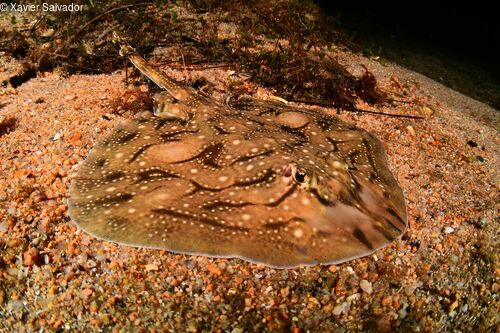
-
Bounding-box search. Observations within a rectangular area
are retrieved by supplying the coordinates of the southwest and
northeast corners. For example, to search around Platja de Sant Sebastià
in Barcelona, define the bounding box and pass it to
mnk_obs().
# read shapefile of  study area using relative path

shp <- "../inst/extdata/espigo_w.shp"

espigo <- sf::st_read(shp, quiet = TRUE)

# ensure WGS84 for leaflet (standard for web maps)

bounds <- st_transform(espigo, 4326)
Similarly, the area can also be defined by a vector from two points, Pmax and Pmin, where the area is defined as:
bounds <- c(ymax, xmax, ymin, xmin)
Applied to the Espigo del W example, this would be:
bounds <-c(41.371239, 2.193971, 41.368182, 2.189147)
The two points, pmax and pmin, will be displayed together with the study area of the Espigo del W in leaflet to help understand how the bounds parameter works.
#Pmin
xmin <- 2.189147
ymin <- 41.368182

#Pmax
xmax <- 2.193971
ymax <- 41.371239

pts <- data.frame(
  id = c("Pmin", "Pmax"),
  lng = c(xmin, xmax),
  lat = c(ymin, ymax)
)

# create interactive map for visualising the study area and the two points

bound <- leaflet() %>%
                addProviderTiles("Esri.WorldImagery", group = "Satélite") %>%
                addProviderTiles("OpenStreetMap", group = "OSM") %>%
                addCircleMarkers(
                         data = pts,
                          radius = 20,
                          color = "cyan",
                          weight = 2,
                          fillOpacity = 0.7,
                          label = ~id,
                          popup = ~paste0("<b>", id, "</b><br>",
                                          "lon: ", round(lng, 6), "<br>",
                                          "lat: ", round(lat, 6))) %>%
                addPolygons(data =    bounds,
                          color = "#2c4fb8",
                          weight = 2,
                          opacity = 1,
                          fillOpacity = 0.4,
                          label = "Bound Espigo W",
                          popup = "Bound Espigo W",
                          highlightOptions = highlightOptions(weight = 3,
                                                              bringToFront =TRUE)) %>%
                addLayersControl(baseGroups = c("Satélite", "OSM"))
#> Assuming "lng" and "lat" are longitude and latitude, respectively

bound  # display map in document
#Obtaining the observations within the study area

obs_torpedo_bounds <- mnk_obs(taxon_name = "Torpedo", year = 2024,
                      bounds = bounds , quality = "research", quiet = TRUE)

obs_torpedo_bounds
#> # A tibble: 7 × 27
#>       id observed_on  year month  week   day  hour created_at         updated_at
#>    <int> <chr>       <int> <int> <int> <int> <int> <chr>              <chr>
#> 1 244605 2024-03-22   2024     3    12    22    20 2024-03-24T18:34:… 2024-03-3…
#> 2 244604 2024-03-22   2024     3    12    22    20 2024-03-24T18:34:… 2024-03-3…
#> 3 244594 2024-03-22   2024     3    12    22    20 2024-03-24T18:34:… 2024-03-3…
#> 4 304290 2024-07-20   2024     7    29    20    18 2024-07-20T18:36:… 2024-07-2…
#> 5 301613 2024-07-16   2024     7    29    16    22 2024-07-17T09:30:… 2024-07-2…
#> 6 315533 2024-08-01   2024     8    31     1     9 2024-08-03T09:08:… 2024-08-0…
#> 7 315527 2024-08-01   2024     8    31     1     9 2024-08-03T09:08:… 2024-08-0…
#> # ℹ 18 more variables: latitude <dbl>, longitude <dbl>,
#> #   positional_accuracy <int>, geoprivacy <chr>, obscured <lgl>, uri <chr>,
#> #   url_picture <chr>, quality_grade <chr>, taxon_id <int>, taxon_name <chr>,
#> #   taxon_rank <chr>, taxon_min_ancestry <chr>, taxon_endemic <lgl>,
#> #   taxon_threatened <lgl>, taxon_introduced <lgl>, taxon_native <lgl>,
#> #   user_id <int>, user_login <chr>

#Turning the dataframe into an sf object with the mnk_obs_sf() function and
#selecting some fields ("id","taxon_name","observed_on",.....) from the original
#data frame for to show later in leaflet popups.

obs_bounds_sf <- mnk_obs_sf(obs_torpedo_bounds,"id","taxon_name","observed_on", "url_picture", "uri", "user_login")

# Preparing the obtained data for later display in the marker popup

popup_final_torpedo <-  paste0( "ID: <a href='", obs_bounds_sf$uri,
                        "' target='_blank'>",obs_bounds_sf$id , "</a><br>",
                        "Specie:", obs_bounds_sf$taxon_name, "<br>",
                        "Observer: ", obs_bounds_sf$user_login,"<br>",
                        "Date:", obs_bounds_sf$observed_on, "<br>",
                        "<a href= '", obs_bounds_sf$url_picture,
                        "' target='_blank'><img src='",
                        obs_bounds_sf$url_picture,
                        "' style='margin-top:2px;border-radius:4px;'> </a> ")

#final plot

bound %>%
  addMarkers(data = obs_bounds_sf, popup = ~popup_final_torpedo)
● mnk_obs_byday()
Works like mnk_obs() but uses an explicit date interval
instead of year or month parameters. The interval is defined by:
d1: start date in ‘yyyy-mm-dd’ format d2:
end date in ‘yyyy-mm-dd’ format
#Retrieves observations for specie Raja undulata by user Xasalva (user_id= 4) the observations between 01-01-2024 and  25-05-2024.

obs_undulata_2024 <- mnk_obs_byday(taxon_name = "Raja undulata", d1 = "2024-01-01",
                             d2= "2024-05-25", quiet = TRUE, quality = "research")

obs_undulata_2024
#> # A tibble: 10 × 29
#>        id observed_on  year month  week   day  hour created_at        updated_at
#>     <int> <chr>       <int> <int> <int> <int> <int> <chr>             <chr>
#>  1 457257 2024-02-17   2024     2     7    17    10 2025-05-20T10:44… 2025-05-2…
#>  2 271165 2024-05-12   2024     5    19    12    11 2024-05-22T20:31… 2025-03-1…
#>  3 270617 2024-05-11   2024     5    19    11    22 2024-05-21T22:52… 2024-05-2…
#>  4 264653 2024-05-08   2024     5    19     8    21 2024-05-09T14:08… 2025-03-1…
#>  5 253086 2024-04-15   2024     4    16    15    19 2024-04-16T18:19… 2024-04-1…
#>  6 232230 2024-02-18   2024     2     7    18    10 2024-02-24T10:38… 2025-03-1…
#>  7 230658 2024-02-18   2024     2     7    18    11 2024-02-19T19:25… 2024-02-2…
#>  8 230538 2024-02-18   2024     2     7    18    10 2024-02-19T14:36… 2024-02-2…
#>  9 229797 2024-02-18   2024     2     7    18    10 2024-02-18T21:41… 2024-02-1…
#> 10 222442 2024-02-03   2024     2     5     3    11 2024-02-06T18:34… 2025-03-1…
#> # ℹ 20 more variables: latitude <dbl>, longitude <dbl>,
#> #   positional_accuracy <int>, geoprivacy <lgl>, obscured <lgl>, uri <chr>,
#> #   photo_url_square <chr>, photo_url_medium <chr>, quality_grade <chr>,
#> #   species_guess <chr>, taxon_id <int>, taxon_name <chr>, taxon_rank <chr>,
#> #   taxon_min_ancestry <chr>, taxon_endemic <lgl>, taxon_threatened <lgl>,
#> #   taxon_introduced <lgl>, taxon_native <lgl>, user_id <int>, user_login <chr>
- Auxiliary functions
The examples below show how the helper functions work. The first two use the Torpedo torpedo observations at the Espigó Hotel W from the previous sections. The last two use separate, specific examples.
● mnk_obs_sf()
This function converts an observations data frame into a spatial
layer in sf format. The function takes the latitude/longitude columns
returned by mnk_obs or by any other function in the rminka
package that returns an observations data frame — such as
mnk_proj_obs or mnk_user_obs — and converts
them into an sf POINT layer. By default the geometry is returned in CRS
EPSG:4326 (WGS84), but you can specify any CRS you need via the crs
argument. Its basic usage has already been shown briefly in previous
sections. Here we develop a detailed example using the Torpedo
torpedo observations at the espigó Hotel W.
obs_utm <- mnk_obs_sf(obs_torpedo_bounds, id, taxon_name,
                      observed_on, user_login, quality_grade, url_picture,
                      uri, crs = 25831)

# The input obs_torpedo_bounds is a data frame with the full set of observation records. The
#function keeps only the selected attribute columns (id, taxon_name, observed_on, user_login,
#quality_grade, url_picture, uri); these are preserved in the output sf object together with
#the generated geometry in obs_utm.

#The crs = 25831 parameter overrides the default EPSG:4326.
#Here we request the output directly in EPSG:25831 – ETRS89 / UTM zone 31N,
#which is the official projected CRS for Catalonia.
#This is useful for distance calculations and for matching local cartography


# Leaflet natively works in Web Mercator (EPSG:3857). To visualize data in UTM,
#you must change the map's base CRS:

crs25831 <- leafletCRS(
  crsClass = "L.Proj.CRS",
  code = "EPSG:25831",
  proj4def = "+proj=utm +zone=31 +ellps=GRS80 +units=m +no_defs",
  resolutions = c(8192,4096,2048,1024,512,256,128,64,32,16,8,4,2,1,0.5),
  origin = c(0, 9000000)
)

# Because the map is no longer in 3857, you cannot use standard OSM tiles.
#You need a WMS that serves imagery in the same CRS.
#Here we use the Institut Cartogràfic i Geològic de Catalunya (ICGC) service.

leaflet(options = leafletOptions(crs25831, minZoom = 0, maxZoom = 14)) %>%

      addWMSTiles(
        "https://geoserveis.icgc.cat/servei/catalunya/mapa-base/wms",
        layers = "orto",
        options = WMSTileOptions(format = "image/png",
                                 transparent = TRUE, version = "1.3.0")) %>%

      addCircleMarkers(
        data = obs_utm,
        radius = 6,
        color = "red",
        fillOpacity = 0.9,
        popup =  paste0( "ID: <a href='", obs_utm$uri,
                            "' target='_blank'>",obs_utm$id , "</a><br>",
                            "Specie:", obs_utm$taxon_name, "<br>",
                            "Observer: ", obs_utm$user_login,"<br>",
                            "Quality:", obs_utm$quality_grade,"<br>",
                            "Date:", obs_utm$observed_on, "<br>",
                            "<a href= '", obs_utm$url_picture,
                            "' target='_blank'><img src='",
                            obs_utm$url_picture,
                            "' style='margin-top:2px;border-radius:4px;'> </a> "))
● export_mnk_qgis()
This function writes one or more sf objects to a GeoPackage (.gpkg), creating one layer per object. It is designed for a smooth GIS workflow ( specialy QGIS): it ensures valid geometries, drops Z/M dimensions, removes list-columns that GDAL cannot write, and transforms features to the target CRS.
We will apply it to the two examples from the previous section.
export_mnk_qgis(observations =obs_utm ,file="shape")

#In this first example we export the observations layer from the previous step (obs_utm)
#as a single point layer named "observations". The output file is named "shape" — the .gpkg
#extension is added automatically.Because no path is specified, the file shape.gpkg is saved
#in the current R working directory of the project.

export_mnk_qgis(zone = places_forum , observations = obs_sf,
                file = "C:/examples/forum.gpkg")

#In the second example export several layers at once. Here we write two layers
#into the same GeoPackage:

# *  places_forum — a polygon defining the Forum pools area, saved as layer "zone"

# * obs_sf — point observations from the Forum pools, saved as layer "observations"
#Both layers are stored in forum.gpkg inside the "examples" folder.
● get_wrm_tax()
This function downloads taxonomic information from the World Register of Marine Species (WoRMS) for a given scientific name. Two examples are provided to illustrate its practical use, particularly when working with tibbles returned by observation functions. In these cases, the goal is to obtain the observations tibble enriched with the complete taxonomy for each recorded species, including its marine,its freshwater, brackish, or extinct status.
#First example – single species

get_wrm_tax("Diplodus sargus")
#> # A tibble: 1 × 14
#>   valid_AphiaID valid_name      rank    kingdom  phylum class order family genus
#>           <int> <chr>           <chr>   <chr>    <chr>  <chr> <chr> <chr>  <chr>
#> 1        127053 Diplodus sargus Species Animalia Chord… Tele… Eupe… Spari… Dipl…
#> # ℹ 5 more variables: isMarine <lgl>, isBrackish <lgl>, isFreshwater <lgl>,
#> #   isTerrestrial <lgl>, isExtinct <lgl>

#The taxonomy and metadata are retrieved for a single species, Diplodus sargus.

#Second example – community taxonomy
#The taxonomy is retrieved for all species observed in the previous `mnk_place_ob`
#call — all species recorded in the Forum pools area during February 2025 (obs_place).

taxon_unic <- obs_place %>%
  filter(!is.na(taxon_name)) %>%
  distinct(taxon_name) %>%
  pull(taxon_name)

taxonomy_df <- map_dfr(
  setNames(taxon_unic, taxon_unic),
  ~ get_wrm_tax(.x),
  .id = "taxon_name"
)
#> No taxon found for the scientific name: 'Life'.
#> No taxon found for the scientific name: 'Ichthyaetus audouinii'.

#The complete observations tibble for the Forum pools can be rebuilt with taxonomy #information by performing a left_join() between obs_place and the taxonomy dataframe.

obs_place_tax <- obs_place %>%
  left_join(taxonomy_df, by = "taxon_name")
● shrt_name()
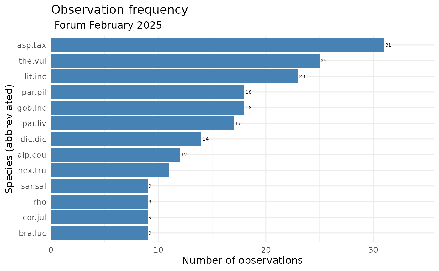
This function creates a standardized abbreviation from a scientific name. In the following example it is used to generate a bar plot of observation frequencies for the species in the “obs_place” tibble, with the abbreviated names making the chart easier to read.
#Create standardized abbreviations for scientific names

obs_place <- obs_place %>%
  mutate(
    shrt_tax_name = map_chr(taxon_name, ~ {
      if (is.na(.x) || .x == "") NA_character_ else shrt_name(.x)
    })
  )

#Count observations per abbreviated species and keep top 10

freq_top10 <- obs_place %>%
  filter(!is.na(shrt_tax_name)) %>%          # remove missing names
  count(shrt_tax_name, name = "n_obs") %>%    # count occurrences
  slice_max(n_obs, n = 10) %>%                # keep the 10 most frequent
  arrange(n_obs)

#Plot horizontal bar chart of observation frequency

ggplot(freq_top10, aes(x = n_obs, y = reorder(shrt_tax_name, n_obs))) +
        geom_col(fill = "steelblue") +
        geom_text(aes(label = n_obs), hjust = -0.2, size = 2) +  # add n as label
        scale_x_continuous(expand = expansion(mult = c(0, 0.15))) +  # make room for labels
        labs(
              x = "Number of observations",
              y = "Species (abbreviated)",
              title = "Observation frequency",
              subtitle = " Forum February 2025"
            ) +
        theme_minimal(base_size = 12)